39 adding labels to excel chart
How to add axis label to chart in Excel? - ExtendOffice You can insert the horizontal axis label by clicking Primary Horizontal Axis Title under the Axis Title drop down, then click Title Below Axis, and a text box will appear at the bottom of the chart, then you can edit and input your title as following screenshots shown. 4. Adding Data Labels to Your Chart (Microsoft Excel) - tips To add data labels, follow these steps: Activate the chart by clicking on it, if necessary. Choose Chart Options from the Chart menu. Excel displays the Chart Options dialog box. Make sure the Data Labels tab is selected. (See Figure 1.) The left side of the dialog box shows the different types of data labels you can choose.
How to Add Data Labels to an Excel 2010 Chart - dummies Select where you want the data label to be placed. Data labels added to a chart with a placement of Outside End. On the Chart Tools Layout tab, click Data Labels→More Data Label Options. The Format Data Labels dialog box appears.
Adding labels to excel chart
Add a DATA LABEL to ONE POINT on a chart in Excel All the data points will be highlighted. Click again on the single point that you want to add a data label to. Right-click and select ' Add data label '. This is the key step! Right-click again on the data point itself (not the label) and select ' Format data label '. You can now configure the label as required — select the content of ... How to Add Axis Label to Chart in Excel - Sheetaki Select the chart that you want to add an axis label. Next, head over to the Chart tab. Click on the Axis Titles. Navigate through Primary Horizontal Axis Title > Title Below Axis. An Edit Title dialog box will appear. In this case, we will input "Month" as the horizontal axis label. Next, click OK. › solutions › excel-chatHow to Insert Axis Labels In An Excel Chart | Excelchat We have a sample chart as shown below; Figure 2 – Adding Excel axis labels. Next, we will click on the chart to turn on the Chart Design tab; We will go to Chart Design and select Add Chart Element; Figure 3 – How to label axes in Excel . In the drop-down menu, we will click on Axis Titles, and subsequently, select Primary Horizontal Figure ...
Adding labels to excel chart. Adding Data Labels to Your Chart (Microsoft Excel) To add data labels in Excel 2013 or Excel 2016, follow these steps: Activate the chart by clicking on it, if necessary. Make sure the Design tab of the ribbon is displayed. (This will appear when the chart is selected.) Click the Add Chart Element drop-down list. Select the Data Labels tool. How do I add axis labels in Excel? - Chariotarot.com How do I add axis labels in Excel? Click the chart, and then click the Chart Design tab. Click Add Chart Element > Axis Titles, and then choose an axis title option. Type the text in the Axis Title box. To format the title, select the text in the title box, and then on the Home tab, under Font, select the formatting that you want. How to Add Axis Labels to a Chart in Excel | CustomGuide Add Data Labels. Use data labels to label the values of individual chart elements. Select the chart. Click the Chart Elements button. Click the Data Labels check box. In the Chart Elements menu, click the Data Labels list arrow to change the position of the data labels. Excel charts: add title, customize chart axis, legend and data labels ... Click the Chart Elements button, and select the Data Labels option. For example, this is how we can add labels to one of the data series in our Excel chart: For specific chart types, such as pie chart, you can also choose the labels location. For this, click the arrow next to Data Labels, and choose the option you want.
Add or remove data labels in a chart - Microsoft Support Add data labels to a chart Click the data series or chart. To label one data point, after clicking the series, click that data point. In the upper right corner, next to the chart, click Add Chart Element > Data Labels. To change the location, click the arrow, and choose an option. Adding Data Labels to Your Chart (Microsoft Excel) Depending on the type of chart you are creating, data labels can mean quite a bit. For instance, if you are formatting a pie chart, the data can be more difficult to understand if you don't include data labels. To add data labels in Excel 2007 or Excel 2010, follow these steps: Activate the chart by clicking on it, if necessary. Adding rich data labels to charts in Excel 2013 - Microsoft 365 Blog One familiar and simple way is just single click on any data value (or column, in this example) to select the entire data series that it belongs to. Above, I have clicked all of the blue columns. Once the series is selected, I can right-click any column to pull up the context menu, then click the Add Data Labels entry. Add data labels and callouts to charts in Excel 365 | EasyTweaks.com The steps that I will share in this guide apply to Excel 2021 / 2019 / 2016. Step #1: After generating the chart in Excel, right-click anywhere within the chart and select Add labels . Note that you can also select the very handy option of Adding data Callouts.
Add / Move Data Labels in Charts - Excel & Google Sheets Adding Data Labels Click on the graph Select + Sign in the top right of the graph Check Data Labels Change Position of Data Labels Click on the arrow next to Data Labels to change the position of where the labels are in relation to the bar chart Final Graph with Data Labels How to Add Labels to Scatterplot Points in Excel - Statology Step 3: Add Labels to Points Next, click anywhere on the chart until a green plus (+) sign appears in the top right corner. Then click Data Labels, then click More Options… In the Format Data Labels window that appears on the right of the screen, uncheck the box next to Y Value and check the box next to Value From Cells. Add label to Excel chart line • AuditExcel.co.za MS Excel Training Adding a label to an Excel line chart is very easy. As shown below, you can create the chart and then right click on the line and choose 'Add Data Labels' and then 'Add Data Labels' again. The labels are immediately put on the chart and Excel has 'guessed' that you wanted the values to appear. However, by right clicking on the ... Adding Data Labels To An Excel Chart | MyExcelOnline In our example below, I add a Data Label to a column chart and then I format the data label using CTRL+1. I then select to custom format the numbers so it shows the values as thousands by adding a comma , after each zero and then showing the work k by adding "k" Example Custom Number Format: [$$-1004]#,##0 ,"k" ;- [$$-1004]#,##0 ,"k"
Adding an horizontal line in excel graph at the origin of secondary axis - Super User
› excel › excel-chartsCreate a multi-level category chart in Excel - ExtendOffice 22. Now the new series is shown as scatter dots and displayed on the right side of the plot area. Select the dots, click the Chart Elements button, and then check the Data Labels box. 23. Right click the data labels and select Format Data Labels from the right-clicking menu. 24. In the Format Data Labels pane, please do as follows.
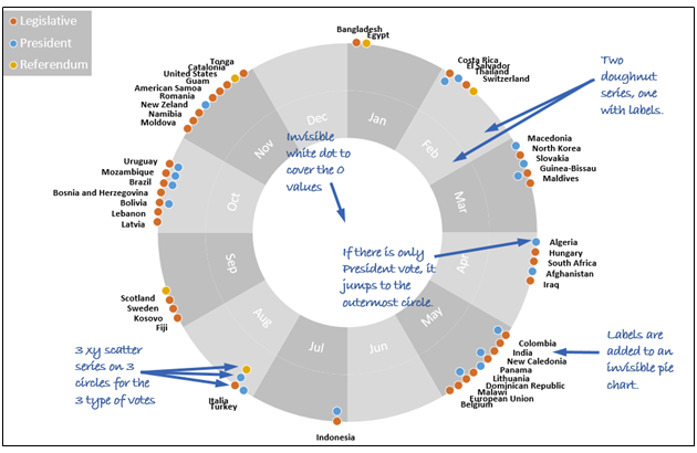
Combine pie and xy scatter charts - Advanced Excel Charting Example | Chandoo.org - Learn ...
trumpexcel.com › dynamic-chart-rangeHow to Create a Dynamic Chart Range in Excel This dynamic range is then used as the source data in a chart. As the data changes, the dynamic range updates instantly which leads to an update in the chart. Below is an example of a chart that uses a dynamic chart range. Note that the chart updates with the new data points for May and June as soon as the data in entered.
Making a Slope Chart or Bump Chart in Excel - How To - PakAccountants.com
› documents › excelHow to wrap X axis labels in a chart in Excel? When the chart area is not wide enough to show it's X axis labels in Excel, all the axis labels will be rotated and slanted in Excel. Some users may think of wrapping the axis labels and letting them show in more than one line. Actually, there are a couple of tricks to warp X axis labels in a chart in Excel. Wrap X axis labels with adding hard ...
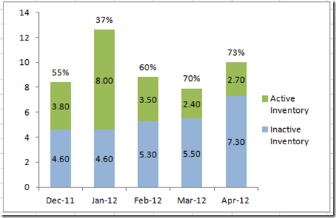
Excel Dashboard Templates How-to Put Percentage Labels on Top of a Stacked Column Chart - Excel ...
How to Use Cell Values for Excel Chart Labels Select the chart, choose the "Chart Elements" option, click the "Data Labels" arrow, and then "More Options." Uncheck the "Value" box and check the "Value From Cells" box. Select cells C2:C6 to use for the data label range and then click the "OK" button. The values from these cells are now used for the chart data labels.

34 How To Label Charts In Excel - Labels Database 2020
Add data labels to your Excel bubble charts | TechRepublic Follow these steps to add the employee names as data labels to the chart: Right-click the data series and select Add Data Labels. Right-click one of the labels and select Format Data Labels. Select...
Budget Calculator Excel Spreadsheet | Budget Calculator
Custom Chart Data Labels In Excel With Formulas Select the chart label you want to change. In the formula-bar hit = (equals), select the cell reference containing your chart label's data. In this case, the first label is in cell E2. Finally, repeat for all your chart laebls. If you are looking for a way to add custom data labels on your Excel chart, then this blog post is perfect for you.
Post a Comment for "39 adding labels to excel chart"